One-Pixel Attacks: Why Computer Vision Security Is Broken

State-of-the-art image classifiers can identify thousands of objects with near-human accuracy. They power self-driving cars, medical diagnostics, and security systems. But a 2019 paper by Su et al. proved something unsettling: you can make these systems completely misclassify an image by changing a single pixel. Not photoshopping the whole thing. Not adding noise everywhere. One pixel out of 50,000+.
The attack works on ResNet, VGG, Inception—pretty much every major CNN architecture. And modern Vision Transformers like ViT aren't safe either. Similar sparse attacks using adversarial patches can fool them just as effectively. The attack doesn't require access to the model's weights or gradients. Just query access and an optimization algorithm called differential evolution.
Here's a concrete example. Take a 224x224 image of a cat—that's 150,528 individual RGB values. The model correctly identifies it as "tabby cat" with 92% confidence. Change the pixel at position (127, 89) from RGB(203, 189, 145) to RGB(67, 23, 198). The model now sees "dog" with 87% confidence. To a human, the images look identical.
This isn't a bug in one specific model. It's a fundamental property of how neural networks operate in high-dimensional space. The decision boundaries between classes are way more fragile than anyone building production vision systems seems to acknowledge.
This post explains what makes single-pixel attacks work, why standard defenses fail, and what the research actually shows about defending against them (spoiler: it's not great). Plus working code so you can test it on actual classifiers.
The Research Behind One-Pixel Attacks
What Su et al. Demonstrated
The seminal work came from Su, Vargas, and Sakurai in 2019. They showed that differential evolution (DE)—an evolutionary optimization algorithm—could find single pixels that cause misclassification across multiple deep neural networks.
Their key findings:
- 70.97% attack success rate on CIFAR-10 against VGG and NiN
- 52.40% success on ImageNet models
- Attacks often transferred between different architectures
- Only required black-box access (no gradients needed)
The paper proved this wasn't a theoretical concern. They tested it on real, deployed architectures. And it worked.
How This Compares to Other Adversarial Attacks
Prior work on adversarial examples mostly used gradient-based methods. Goodfellow et al.'s FGSM (2014) perturbs all pixels slightly using gradient information. Madry et al.'s PGD (2017) uses iterative gradient ascent. The Carlini & Wagner attack (2017) is optimization-based but still perturbs all pixels.
These attacks needed access to gradients (white-box) or perturbed many pixels. One-pixel attacks are different. They're black-box—only need model predictions. They're extremely sparse—literally one pixel. And they use evolutionary optimization instead of gradients.
Why This Matters for Security
The attack surface is massive. A 224x224 image has 50,176 pixels. Each has 3 color channels (RGB) with 256 possible values. That's roughly 50,000 locations × 16 million color combinations. An attacker only needs to find one that works.
Real-world implications:
Autonomous vehicles: A small physical perturbation—a sticker on a sign—could be one "pixel" from the camera's perspective.
Medical imaging: Subtle manipulation in a diagnostic image could cause misdiagnosis. Finlayson et al. (2019) showed adversarial attacks work on medical imaging systems and are extremely difficult to detect.
Security systems: Facial recognition defeated by a tiny modification humans can't perceive.
Content moderation: Harmful content sneaks past filters with an imperceptible change.
Why defenses are hard: You can't sanitize an image by "removing bad pixels"—there are millions of possibilities to check. Human review doesn't help because the changes are imperceptible. And the attacks often transfer across models, so ensemble defenses only partially work.
Beyond CNNs: Vision Transformers Are Vulnerable Too
The original Su et al. work focused on convolutional neural networks (ResNet, VGG, Inception). But computer vision has evolved. Vision Transformers (ViTs) now dominate many benchmarks, replacing CNNs in production systems.
Are ViTs more robust?
Early work by Mahmood et al. (2021) suggested ViTs might have better adversarial robustness than CNNs due to their self-attention mechanism capturing global interactions rather than local patterns. This seemed promising.
The reality is more nuanced. Recent research shows ViTs are vulnerable to sparse adversarial attacks, sometimes even more so than CNNs.
Joshi et al. (2021) demonstrated "adversarial token attacks" where modifying just a few patches (16x16 tokens) can fool ViTs. The patch-based architecture that seemed like a strength becomes a vulnerability.
Wei et al. (2022) showed ViTs can be attacked with minimal perturbations using patch-specific strategies. Their "Patch-Fool" attack found ViTs are more vulnerable than CNNs when perturbations target individual patches at high density.
Naseer et al. (2021) found that while gradient-based attacks transfer less effectively to ViTs, targeted attacks that account for the attention mechanism work extremely well.
Why ViTs are vulnerable differently: The self-attention mechanism operates on patches. An adversarial perturbation doesn't need to be spread across the entire image—it can concentrate in a few patches that will influence the attention mechanism. This is conceptually similar to the one-pixel attack but operates at the patch level.
A single adversarial patch (16x16 pixels in a standard ViT) can corrupt the global attention computation, causing cascading failures in the model's understanding of the image.
The Bigger Pattern
This vulnerability isn't unique to computer vision. It's part of a broader pattern in ML security:
- LLMs: Can't distinguish system prompts from user input (prompt injection)
- Computer vision: Can't distinguish adversarial perturbations from legitimate data—across both CNNs and transformers
- RL systems: Optimize for metrics rather than intended goals (reward hacking)
The common thread: ML systems optimize for average-case performance on training distributions, not worst-case robustness against adversarial inputs. Architectural innovations (transformers vs CNNs) don't fundamentally solve this problem.
How the Attack Actually Works
Understanding the Vulnerability
Image classifiers learn to draw boundaries in high-dimensional space. On one side of the boundary, images are "cat." On the other side, "dog." The problem is these boundaries aren't smooth. They're jagged, complex surfaces with lots of near-boundary regions.
A single pixel change in the input can cause a large change in the model's internal representations (feature space). If the image is near a decision boundary, that large feature change can push it across.
The Differential Evolution Approach
Why use evolutionary optimization?
Gradient-based attacks need access to the model's gradients—how the loss changes with each input pixel. Many deployed models don't expose this. They just give you predictions.
Differential Evolution (DE) is a black-box optimization algorithm from Storn and Price (1997). It treats the model as a black box—just queries it and uses the predictions to guide search.
How DE works (simplified):
- Initialize population: Generate random candidate solutions (pixel modifications)
- Evaluate fitness: Apply each modification, check if model is fooled
- Mutation & crossover: Create new candidates by combining successful ones
- Selection: Keep the best performers
- Iterate: Repeat until you find an adversarial example or hit max iterations
Why it works for this problem:
- Only 5 parameters to optimize (x, y, R, G, B)
- No gradients needed, just model predictions
- Good at finding global optima in complex search spaces
- Naturally handles discrete variables (pixel coordinates)
Attack Parameters and Search Space
What you're searching for:
- Pixel x-coordinate: 0 to 223 (for 224x224 image)
- Pixel y-coordinate: 0 to 223
- New R value: 0 to 255
- New G value: 0 to 255
- New B value: 0 to 255
That's roughly 224 × 224 × 256³ = ~1.9 trillion possible single-pixel modifications. Brute force won't work. But DE can efficiently search this space.
The Attack Algorithm
Input: Original image, target model, max iterations
Output: Adversarial image (or failure)

1. Get original classification and confidence
2. Initialize DE population:
   - Generate N random (x, y, r, g, b) tuples
   - Each represents a single-pixel modification
3. For each iteration:
   a. Evaluate population:
      - Apply each modification to original image
      - Get model's prediction
      - Compute fitness (lower confidence in original class = better)
   b. If any modification causes misclassification:
      - Return adversarial image
   c. Otherwise:
      - Mutation: Create variants by perturbing good candidates
      - Crossover: Combine parameters from different candidates
      - Selection: Keep best N candidates for next generation
4. If max iterations reached without success:
   - Return failure

Typical success: 50-100 iterations for vulnerable images
Why This Works Against Modern Classifiers
The black-box advantage: Most deployed models expose only a prediction API. The attack doesn't need model architecture details, training data, weight values, or gradient information. It only needs to query the model and see predictions. This makes it practical against real-world systems.
Transferability: Su et al. found that adversarial examples often work across different models. An attack crafted for ResNet might also fool VGG or Inception. This is because different architectures often learn similar vulnerable decision boundaries.
Testing It Yourself
A Note on Image Resolution
The examples in this section use CIFAR-10 images rather than photos from your phone or ImageNet. This is intentional, and worth understanding why.
Su et al.'s 70.97% success rate was measured on CIFAR-10—32×32 pixel images with 3,072 total values. Their ImageNet results were considerably lower at 52.40%, and in practice attacking higher-resolution images is significantly harder. The reason comes back to the dimensionality argument: a single pixel represents roughly 1-in-3,000 of a CIFAR-10 image, versus 1-in-150,000 of a 224×224 image. The search space for DE doesn't change (still just 5 parameters), but the perturbation's influence on the model's internal representations is proportionally much smaller at higher resolution. Decision boundaries in 150,000-dimensional space have a lot more room between them.
This means if you try to reproduce this attack on arbitrary high-resolution photos, you'll likely see it fail. That's not a bug in the implementation—it's a meaningful finding about real-world applicability. The attack is a genuine vulnerability, but image resolution is a significant moderating factor that the headline numbers don't always make clear.
CIFAR-10 is also convenient: it's built into torchvision, requires no external files, and lets you run across the full 10,000-image test set to measure success rates yourself.
Implementation Setup
Requirements:
- Python 3.8+
- PyTorch (for pre-trained models)
- SciPy (for differential_evolution)
- NumPy, Matplotlib
Installation:
pip install torch torchvision scipy matplotlib numpy
Complete Working Code
Step 1: Load model and dataset
import torch
import torchvision
import torchvision.transforms as transforms
import numpy as np
import matplotlib.pyplot as plt
from scipy.optimize import differential_evolution

# CIFAR-10 class labels
CLASSES = ['airplane', 'automobile', 'bird', 'cat', 'deer',
           'dog', 'frog', 'horse', 'ship', 'truck']

# Load CIFAR-10 test set
# Downloads automatically on first run (~170MB)
transform = transforms.Compose([
    transforms.ToTensor(),
    transforms.Normalize(
        mean=[0.4914, 0.4822, 0.4465],
        std=[0.2023, 0.1994, 0.2010]
    )
])

testset = torchvision.datasets.CIFAR10(
    root='./data', train=False, download=True, transform=transform
)

# Load a pretrained ResNet20 trained on CIFAR-10 (~92% test accuracy)
# torchvision's built-in ResNet weights are ImageNet-only (1000 classes)—don't use those here
model = torch.hub.load(
    "chenyaofo/pytorch-cifar-models",
    "cifar10_resnet20",
    pretrained=True
)
model.eval()
Step 2: Define attack functions
def predict(image_np):
    """
    Get model's prediction for a raw uint8 numpy image (32x32x3).
    Applies normalization internally.
    """
    # Convert to float tensor and normalize
    img = torch.from_numpy(image_np).float() / 255.0
    img = img.permute(2, 0, 1)  # HWC -> CHW
    img[0] = (img[0] - 0.4914) / 0.2023
    img[1] = (img[1] - 0.4822) / 0.1994
    img[2] = (img[2] - 0.4465) / 0.2010
    img = img.unsqueeze(0)

    with torch.no_grad():
        output = model(img)
        probs = torch.nn.functional.softmax(output[0], dim=0)

    top_prob, top_class = torch.max(probs, 0)
    return top_class.item(), top_prob.item(), probs

def perturb_image(image_np, x, y, r, g, b):
    """Apply a single-pixel modification to a numpy image."""
    adversarial = image_np.copy()
    adversarial[int(y), int(x)] = [int(r), int(g), int(b)]
    return adversarial

def attack_objective(params, image_np, original_class):
    """
    Objective function for differential evolution.
    We minimize confidence in the original class.
    Returns negative confidence in wrong class if misclassified
    (lower is better for DE).
    """
    x, y, r, g, b = params
    adversarial = perturb_image(image_np, x, y, r, g, b)
    pred_class, confidence, probs = predict(adversarial)

    if pred_class != original_class:
        return -confidence  # Successfully fooled—return negative confidence
    return probs[original_class].item()  # Still correct—return confidence to minimize
Step 3: Execute the attack
def one_pixel_attack(image_np, original_class, max_iterations=100):
    """
    Run one-pixel attack on a 32x32 CIFAR-10 image.

    Args:
        image_np: uint8 numpy array of shape (32, 32, 3)
        original_class: ground truth class index
        max_iterations: DE generation limit

    Returns:
        adversarial_image, pixel_location (x, y), success bool
    """
    height, width = image_np.shape[:2]

    bounds = [
        (0, width - 1),   # x coordinate
        (0, height - 1),  # y coordinate
        (0, 255),         # R value
        (0, 255),         # G value
        (0, 255)          # B value
    ]

    result = differential_evolution(
        attack_objective,
        bounds,
        args=(image_np, original_class),
        maxiter=max_iterations,
        popsize=10,        # 10 × 5 params = 50 candidates per generation
        recombination=0.7,
        mutation=0.5,      # Fixed mutation factor—works better than a range for 5D
        seed=42,
        polish=False,
        disp=False
    )

    x, y, r, g, b = result.x
    adversarial = perturb_image(image_np, x, y, r, g, b)
    adv_class, adv_conf, _ = predict(adversarial)
    success = (adv_class != original_class)

    return adversarial, (int(x), int(y)), success


# Load raw dataset (no transform—we want uint8 numpy arrays)
raw_dataset = torchvision.datasets.CIFAR10(
    root='./data', train=False, download=False,
    transform=None
)

# Find a good candidate image before running the attack
def find_candidate(dataset, target_conf_min=0.60, target_conf_max=0.85):
    """
    Scan the test set for correctly-classified images with moderate confidence.
    High-confidence images (>90%) sit far from decision boundaries and are
    much harder to attack with a single pixel—DE has almost no signal to follow.
    Images in the 60-85% range are closer to the boundary and attack readily.
    """
    for i in range(len(dataset)):
        image_pil, label = dataset[i]
        image_np = np.array(image_pil)
        pred_class, pred_conf, _ = predict(image_np)

        if pred_class == label and target_conf_min < pred_conf < target_conf_max:
            print(f"Image {i}: {CLASSES[pred_class]} ({pred_conf:.2%}) — good candidate")
            return image_np, label, i

    return None

image_np, label, idx = find_candidate(raw_dataset)
original_class, original_conf, _ = predict(image_np)
print(f"Original: {CLASSES[original_class]} ({original_conf:.2%} confidence)")

adv_img, pixel_loc, success = one_pixel_attack(image_np, original_class)
adv_class, adv_conf, _ = predict(adv_img)

print(f"Adversarial: {CLASSES[adv_class]} ({adv_conf:.2%} confidence)")
print(f"Attack {'succeeded' if success else 'failed'}")
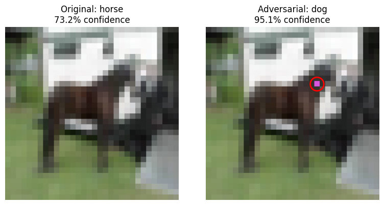
Step 4: Visualize results
fig, axes = plt.subplots(1, 2, figsize=(8, 4))

# Upscale for visibility—32x32 is tiny on screen
display_orig = image_np.repeat(8, axis=0).repeat(8, axis=1)
display_adv = adv_img.repeat(8, axis=0).repeat(8, axis=1)

axes[0].imshow(display_orig)
axes[0].set_title(f'Original: {CLASSES[original_class]}\n{original_conf:.1%} confidence')
axes[0].axis('off')

axes[1].imshow(display_adv)
axes[1].set_title(f'Adversarial: {CLASSES[adv_class]}\n{adv_conf:.1%} confidence')
axes[1].axis('off')

# Scale pixel location to match upscaled display
px, py = pixel_loc
circle = plt.Circle((px * 8 + 4, py * 8 + 4), radius=10,
                     color='red', fill=False, linewidth=2)
axes[1].add_patch(circle)

plt.tight_layout()
plt.savefig('one_pixel_attack_result.png', dpi=300, bbox_inches='tight')
plt.show()
You can view a full working demo on Google Colab here: One Pixel Attacks In Python.
Confidence as a Proxy for Decision Boundary Distance
Before running the attack, it's worth understanding why candidate selection matters.
A classifier's output confidence is a rough proxy for how far an image sits from the nearest decision boundary. When a model says "airplane: 99.8%", it's distributing almost no probability mass to any other class. In the model's feature space, that image is deep inside the "airplane" region—far from the boundary where it might tip over to "ship" or "bird." A single pixel change perturbs the image by a tiny amount in that space. It's not enough to cross the boundary.
An image classified at 65% confidence is a different situation. The model is less certain, which geometrically means the image is closer to a boundary. The remaining 35% probability is distributed across other classes, and some of those classes are nearby in feature space. A single pixel—which represents a meaningful fraction of a 32×32 image—may be enough to push it across.
This is why if you grab raw_dataset[0] and it comes back at 100% confidence, the attack will fail reliably. It's not a bug in the implementation. The find_candidate function above scans for images in the 60–85% confidence range, which are genuinely close to decision boundaries and attack readily.
Su et al.'s 70.97% success rate reflects this distribution across the full CIFAR-10 test set—high-confidence images dragging the number down, low-confidence images pushing it up. If you filter to only images below 80% confidence, you'll see considerably higher success rates.
What to Expect
On a good candidate image, the attack typically succeeds within 50–100 generations. Some will fold in 20. The modified image looks identical to a human—at 32×32, the changed pixel is literally one dot. The model's confidence can swing from 70%+ correct to 80%+ wrong.
Try looping over the first 200 test images and tracking success rate against original confidence. The correlation is clear and makes for an interesting chart—and it's a more honest characterization of the attack than a single cherry-picked success.
Why Defenses Fail
The Fundamental Problem
High-dimensional spaces are weird. Even a CIFAR-10 image lives in 3,072 dimensions (32×32×3). A 224×224 ImageNet image lives in 150,528. In either case, geometric intuition breaks down. What looks like a small perturbation in pixel space can be a huge jump in feature space—and the higher the resolution, the larger and more complex those spaces become. This is why the attack success rate drops from 70% on CIFAR-10 to 52% on ImageNet: more dimensions means more room between decision boundaries, and harder optimization problems for DE to solve.
Neural networks learn complex, non-linear decision boundaries in this space. These boundaries have lots of vulnerable regions—places where tiny input changes cause large representation changes.
Attempted Defenses and Their Limitations
Input preprocessing:
The idea: Apply JPEG compression, blurring, or resizing to destroy perturbations.
The problem: Also destroys legitimate image features. Attackers can adapt by crafting perturbations that survive preprocessing.
Research by Athalye et al. (2018) showed "obfuscated gradients" give a false sense of security. Preprocessing defenses often fail against adaptive attacks.
Adversarial training:
The idea: Include adversarial examples in training to make the model robust.
The problem: Computationally expensive. Only provides robustness against attacks similar to training attacks. Su et al.'s DE-based approach is fundamentally different from gradient-based attacks used in adversarial training.
Madry et al. (2017) showed this helps against FGSM/PGD, but robustness doesn't generalize well to novel attack types.
Defensive distillation:
The idea: Train model to output soft labels (probability distributions) instead of hard predictions.
The problem: Only effective against gradient-based attacks that rely on hard labels. Black-box attacks like one-pixel don't care about gradient characteristics.
Carlini & Wagner (2017) demonstrated this defense could be broken with stronger attacks.
Ensemble defenses:
The idea: Use multiple models. Attack must fool all of them.
The problem: Due to transferability, adversarial examples often work across multiple architectures. Helps a little, but doesn't solve the problem.
Tramèr et al. (2017) found ensembles increase robustness marginally but can still be defeated.
What Actually Provides Some Robustness
Certified defenses work in limited scope. Researchers have developed provably robust networks for small images and perturbations. These provide mathematical guarantees but only work in constrained settings: small images (32×32, not 224×224), small perturbation budgets, and with significant accuracy drops on clean images.
Input validation can catch some attacks by rejecting images with statistical anomalies. But this requires knowing what anomalies to look for—and attackers can adapt.
Human-in-the-loop remains the best defense for high-stakes applications. For medical diagnosis and autonomous vehicles, human oversight makes attacks more expensive and risky. The human doesn't see the perturbation either, but adding a human checkpoint changes the threat model.
The Current State
The research consensus: we don't have practical defenses against adversarial examples that maintain model accuracy. The problem is fundamentally hard. As Ilyas et al. (2019) put it: adversarial vulnerability is "a direct result of sensitivity to well-generalizing features in the data"—in other words, adversarial examples may not be bugs, but rather features of how models learn from high-dimensional data.
Implications and Open Problems
Real-World Attack Scenarios
The one-pixel attack translates to physical scenarios. Researchers have demonstrated adversarial patches on stop signs that cause misclassification (Eykholt et al., 2018), 3D-printed objects that fool classifiers from any angle (Athalye et al., 2018), and adversarial eyeglasses that defeat facial recognition (Sharif et al., 2016).
A small sticker on a physical object can act as a "one-pixel" perturbation from the camera's perspective.
In medical imaging, adversarial perturbations could cause cancer to be misdiagnosed as benign, healthy scans flagged as diseased, or incorrect organ segmentation. Finlayson et al. (2019) showed adversarial attacks work on medical imaging systems and are extremely difficult to detect.
The Broader ML Security Picture
This vulnerability pattern appears across ML domains. In NLP, there's prompt injection in LLMs. In computer vision, adversarial examples. In speech recognition, adversarial audio commands. In reinforcement learning, reward hacking.
The common thread: ML systems aren't designed with security-first principles. They optimize for average-case performance, not worst-case robustness.
Open Research Questions
Still unsolved:
- Can we build provably robust classifiers for realistic image sizes?
- Is there a fundamental tradeoff between accuracy and robustness?
- Can we detect adversarial examples reliably without knowing the attack method?
- How do we deploy vision systems in safety-critical applications?
Active research directions:
- Formal verification techniques
- Certified training methods
- Alternative architectures less vulnerable to adversarial examples
- Better understanding of decision boundary geometry
But practical, deployable solutions don't exist yet.
Practical Guidance
For ML engineers deploying vision systems: Don't deploy in safety-critical contexts without human oversight. Test against adversarial attacks during development. Monitor for input anomalies in production. Understand your model's vulnerabilities before deployment.
For security researchers: This remains an active, important area. New attack variants keep emerging. Defenses that work for one attack often fail for others. Cross-disciplinary work combining ML, security, and formal methods is needed.
Conclusion
The one-pixel attack reveals a fundamental fragility in computer vision systems. State-of-the-art models can be completely fooled by changing a single pixel out of tens of thousands. The attack is easy to execute (differential evolution handles the hard part), hard to defend against (standard countermeasures fail), and works across different architectures—from CNNs to modern Vision Transformers.
This isn't a bug in a specific model. It's a property of how neural networks learn decision boundaries in high-dimensional spaces. Those boundaries are way more brittle than the impressive accuracy numbers suggest.
Current vision systems aren't robust enough for safety-critical applications without human oversight. If you're deploying these models in production, you need to understand their vulnerabilities. Test against adversarial attacks. Have contingency plans. Don't assume "state-of-the-art accuracy" means "secure."
The research community is working on this. But we're years away from practical defenses that maintain accuracy.
The code in this post lets you test it yourself. Try it on your own models. See how vulnerable they are. Then decide if you really want to deploy them without safeguards.
Find This Useful?

References
- Su, J., Vargas, D. V., & Sakurai, K. (2019). "One pixel attack for fooling deep neural networks." IEEE Transactions on Evolutionary Computation, 23(5), 828-841.
- Goodfellow, I. J., Shlens, J., & Szegedy, C. (2014). "Explaining and harnessing adversarial examples." arXiv:1412.6572.
- Carlini, N., & Wagner, D. (2017). "Towards evaluating the robustness of neural networks." IEEE Symposium on Security and Privacy.
- Madry, A., Makelov, A., Schmidt, L., Tsipras, D., & Vladu, A. (2017). "Towards deep learning models resistant to adversarial attacks." ICLR.
- Athalye, A., Engstrom, L., Ilyas, A., & Kwok, K. (2018). "Synthesizing robust adversarial examples." ICML.
- Eykholt, K., Evtimov, I., Fernandes, E., Li, B., Rahmati, A., Xiao, C., Prakash, A., Kohno, T., & Song, D. (2018). "Robust physical-world attacks on deep learning visual classification." CVPR.
- Tramèr, F., Kurakin, A., Papernot, N., Goodfellow, I., Boneh, D., & McDaniel, P. (2017). "Ensemble adversarial training: Attacks and defenses." arXiv:1705.07204.
- Finlayson, S. G., Bowers, J. D., Ito, J., Zittrain, J. L., Beam, A. L., & Kohane, I. S. (2019). "Adversarial attacks on medical machine learning." Science, 363(6433), 1287-1289.
- Ilyas, A., Santurkar, S., Tsipras, D., Engstrom, L., Tran, B., & Madry, A. (2019). "Adversarial examples are not bugs, they are features." NeurIPS.
- Mahmood, K., Mahmood, R., & Van Dijk, M. (2021). "On the Robustness of Vision Transformers to Adversarial Examples." ICCV.
- Joshi, A., Jagatap, G., & Hegde, C. (2021). "Adversarial Token Attacks on Vision Transformers." arXiv:2110.04337.
- Wei, X., Guo, Y., Li, J., & Yu, J. (2022). "Patch-Fool: Are Vision Transformers Always Robust Against Adversarial Perturbations?" ICLR.
- Naseer, M., Ranasinghe, K., Khan, S., Khan, F. S., & Porikli, F. (2021). "Towards Transferable Adversarial Attacks on Vision Transformers." arXiv:2109.04176.
- Storn, R., & Price, K. (1997). "Differential evolution–a simple and efficient heuristic for global optimization over continuous spaces." Journal of Global Optimization, 11(4), 341-359.
- Sharif, M., Bhagavatula, S., Bauer, L., & Reiter, M. K. (2016). "Accessorize to a crime: Real and stealthy attacks on state-of-the-art face recognition." ACM SIGSAC Conference on Computer and Communications Security.